3 Tumors

# ~~~~~~~~~~~~~~~~~~~~~~~~~~~~~~~~~~~ Thu Mar  4 14:23:11 2021
# ggplot theme setup
# ~~~~~~~~~~~~~~~~~~~~~~~~~~~~~~~~~~~ Thu Mar  4 14:23:17 2021

my_theme <- list(
  ggplot2::theme(
    axis.title.x = element_text(colour = "black", size = 16),
    axis.text.x = element_text(size = 14),
    axis.title.y = element_text(colour = "black", size = 16),
    axis.text.y = element_text(size = 14),
    legend.position = "top",
    legend.title = element_blank(),
    legend.text = element_text(size = 14)
  )
)

3.1 TN1

# ~~~~~~~~~~~~~~~~~~~~~~~~~~~~~~~~~~~ Tue Nov 24 17:13:42 2020
# Tumors Heatmaps/Consensus/Trees
# ~~~~~~~~~~~~~~~~~~~~~~~~~~~~~~~~~~~ Tue Nov 24 17:13:47 2020

TN1_ploidy <- 3.45

TN1_popseg <- readRDS(here("extdata/popseg/TN1_popseg.rds"))

TN1_popseg_long_ml <- readRDS(here("extdata/merge_levels/TN1_popseg_long_ml.rds"))

TN1_umap <- run_umap(TN1_popseg_long_ml)

## Constructing UMAP embedding.

TN1_clustering <- run_clustering(TN1_umap,
                                 k_snn_major = 45,
                                 k_snn_minor = 17)

## Loading required package: SingleCellExperiment

## Building SNN graph.

## Running hdbscan.

##  cluster   n    percent
##       c1  32 0.02909091
##      c10  24 0.02181818
##      c11  45 0.04090909
##      c12  19 0.01727273
##      c13  79 0.07181818
##      c14  23 0.02090909
##      c15  51 0.04636364
##      c16  23 0.02090909
##      c17 149 0.13545455
##       c2  56 0.05090909
##       c3 134 0.12181818
##       c4  66 0.06000000
##       c5  40 0.03636364
##       c6  39 0.03545455
##       c7  74 0.06727273
##       c8 228 0.20727273
##       c9  18 0.01636364

## Done.

TN1_ordered <- order_dataset(popseg_long = TN1_popseg_long_ml,
                             clustering = TN1_clustering)

plot_umap(umap_df = TN1_umap,
          clustering = TN1_clustering)

## Joining, by = "cells"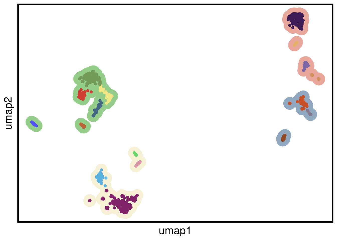

TN1_consensus <- calculate_consensus(df = TN1_ordered$dataset_ordered,
                                     clusters = TN1_ordered$clustering_ordered$subclones)

TN1_gen_classes <- consensus_genomic_classes(TN1_consensus,
                                             ploidy_VAL = TN1_ploidy)

TN1_me_consensus_tree <- run_me_tree(consensus_df = TN1_consensus,
                                     clusters = TN1_clustering,
                                     ploidy_VAL = TN1_ploidy)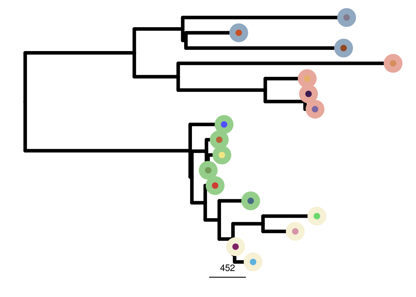

TN1_annotation_genes <- c("SHC1",
                          "RUVBL1",
                          "PIK3CA",
                          "FGFR4",
                          "CDKN1A",
                          "EGFR",
                          "FGFR1",
                          "MYC",
                          "CDKN2A",
                          "GATA3",
                          "PTEN",
                          "CDK4",
                          "MDM2",
                          "BRCA2",
                          "RB1",
                          "TP53",
                          "BRCA1",
                          "CCNE1",
                          "AURKA",
                          "CCND1")

plot_heatmap(df = TN1_ordered$dataset_ordered,
             ploidy_VAL = TN1_ploidy,
             ploidy_trunc = 2*(round(TN1_ploidy)),
             clusters = TN1_ordered$clustering_ordered,
             genomic_classes = TN1_gen_classes,
             keep_gene = TN1_annotation_genes,
             tree_order = TN1_me_consensus_tree$cs_tree_order,
             show_legend = TRUE)

## 'select()' returned 1:1 mapping between keys and columns

## Warning: The input is a data frame, convert it to the matrix.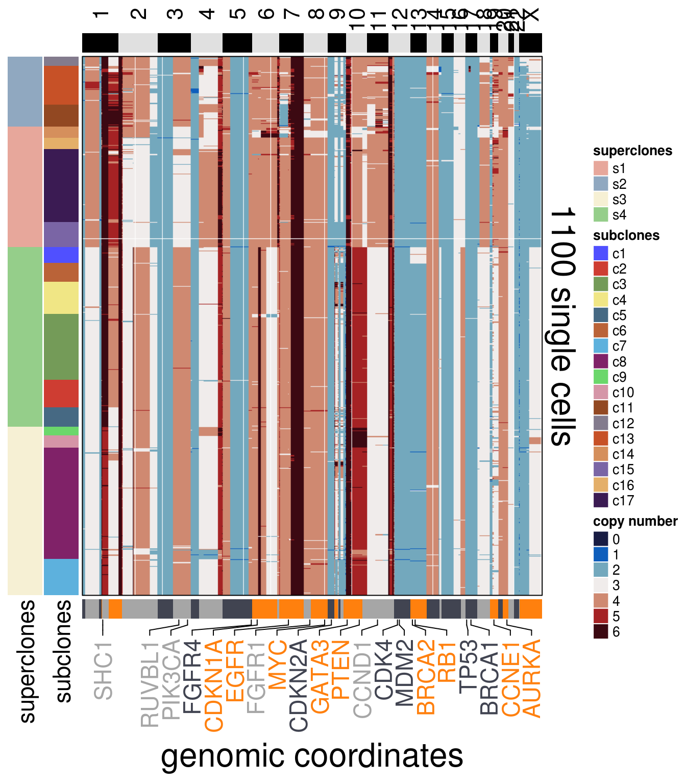

plot_consensus_heatmap(df = TN1_consensus,
                       clusters = TN1_ordered$clustering_ordered,
                       ploidy_VAL = TN1_ploidy,
                       ploidy_trunc = 2*(round(TN1_ploidy)),
                       keep_gene = TN1_annotation_genes,
                       tree_order = TN1_me_consensus_tree$cs_tree_order,
                       plot_title = NULL,
                       genomic_classes = TN1_gen_classes)

## Warning: Setting row names on a tibble is deprecated.

## 'select()' returned 1:1 mapping between keys and columns

## Warning: The input is a data frame, convert it to the matrix.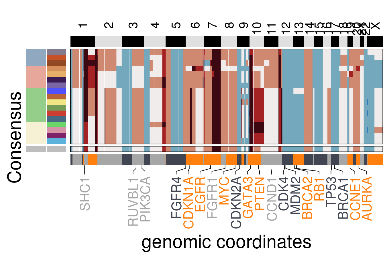

3.2 TN2

# ~~~~~~~~~~~~~~~~~~~~~~~~~~~~~~~~~~~ Tue Nov 24 17:13:42 2020
# Tumors Heatmaps/Consensus/Trees
# ~~~~~~~~~~~~~~~~~~~~~~~~~~~~~~~~~~~ Tue Nov 24 17:13:47 2020

TN2_ploidy <- 3.03

TN2_popseg <- readRDS(here("extdata/popseg/TN2_popseg.rds"))

TN2_popseg_long_ml <- readRDS(here("extdata/merge_levels/TN2_popseg_long_ml.rds"))

TN2_umap <- run_umap(TN2_popseg_long_ml)

## Constructing UMAP embedding.

TN2_clustering <- run_clustering(TN2_umap,
                                 k_snn_major = 63,
                                 k_snn_minor = 17)

## Building SNN graph.

## Running hdbscan.

##  cluster   n    percent
##       c1  23 0.02246094
##      c10 147 0.14355469
##      c11  31 0.03027344
##      c12 140 0.13671875
##      c13  43 0.04199219
##      c14  34 0.03320312
##      c15 156 0.15234375
##       c2  22 0.02148438
##       c3  55 0.05371094
##       c4  51 0.04980469
##       c5  44 0.04296875
##       c6  44 0.04296875
##       c7  28 0.02734375
##       c8 170 0.16601562
##       c9  36 0.03515625

## Done.

TN2_ordered <- order_dataset(popseg_long = TN2_popseg_long_ml,
                             clustering = TN2_clustering)

plot_umap(umap_df = TN2_umap,
          clustering = TN2_clustering)

## Joining, by = "cells"

TN2_consensus <- calculate_consensus(df = TN2_ordered$dataset_ordered,
                                     clusters = TN2_ordered$clustering_ordered$subclones)

TN2_gen_classes <- consensus_genomic_classes(TN2_consensus,
                                             ploidy_VAL = TN2_ploidy)

TN2_me_consensus_tree <- run_me_tree(consensus_df = TN2_consensus,
                                     clusters = TN2_clustering,
                                     ploidy_VAL = TN2_ploidy)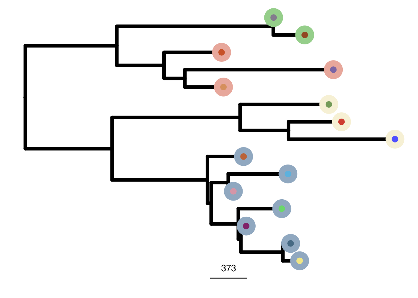

TN2_annotation_genes <- c(
  "SHC1",
  "PIK3CA",
  "FGFR4",
  "CDKN1A",
  "EGFR",
  "MTDH",
  "MYC",
  "GATA3",
  "PTEN",
  "CCND1",
  "PGR",
  "CDK4",
  "MDM2",
  "LRP1B",
  "BRCA2",
  "TP53",
  "BRCA1",
  "BCL2",
  "CCNE1",
  "AURKA"
)

plot_heatmap(df = TN2_ordered$dataset_ordered,
             ploidy_VAL = TN2_ploidy,
             ploidy_trunc = 2*(round(TN2_ploidy)),
             clusters = TN2_ordered$clustering_ordered,
             genomic_classes = TN2_gen_classes,
             keep_gene = TN2_annotation_genes,
             tree_order = TN2_me_consensus_tree$cs_tree_order,
             show_legend = TRUE)

## 'select()' returned 1:1 mapping between keys and columns

## Warning: The input is a data frame, convert it to the matrix.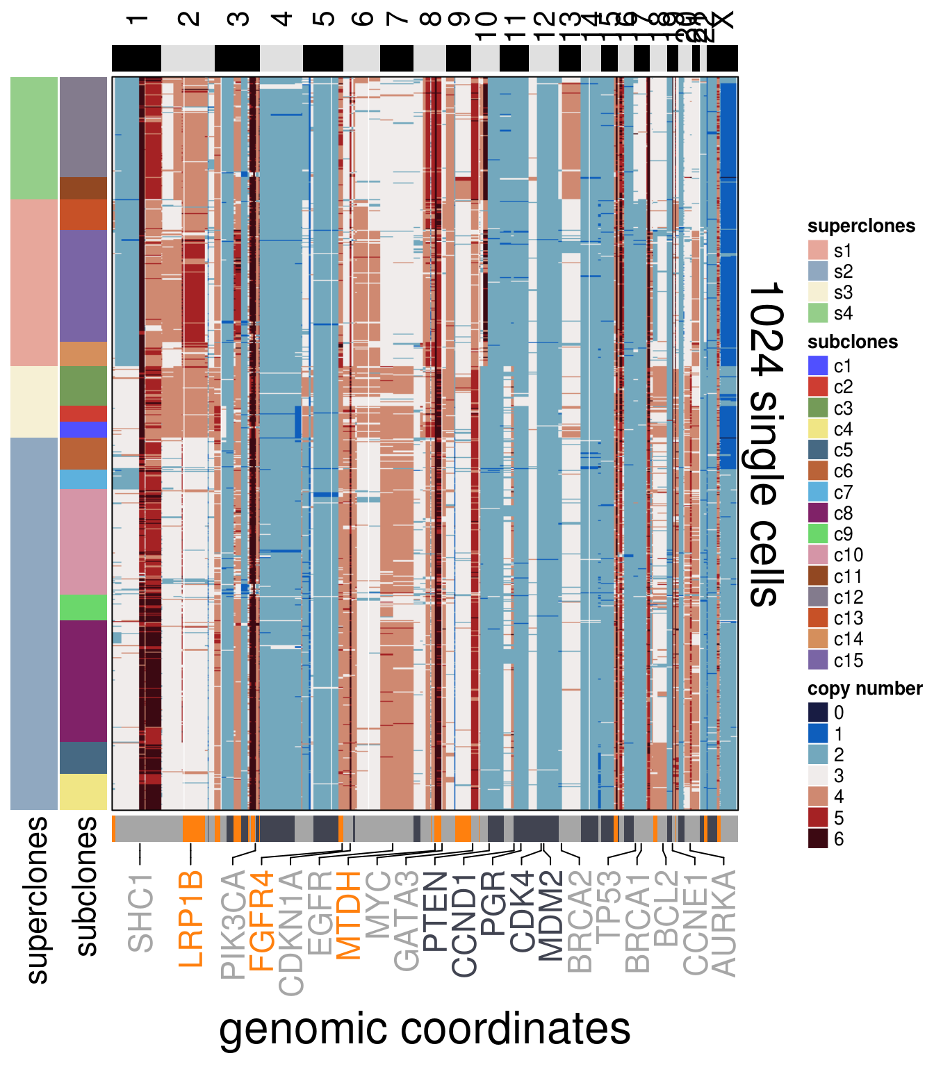

plot_consensus_heatmap(df = TN2_consensus,
                       clusters = TN2_ordered$clustering_ordered,
                       ploidy_VAL = TN2_ploidy,
                       ploidy_trunc = 2*(round(TN2_ploidy)),
                       keep_gene = TN2_annotation_genes,
                       tree_order = TN2_me_consensus_tree$cs_tree_order,
                       plot_title = NULL,
                       genomic_classes = TN2_gen_classes)

## Warning: Setting row names on a tibble is deprecated.

## 'select()' returned 1:1 mapping between keys and columns

## Warning: The input is a data frame, convert it to the matrix.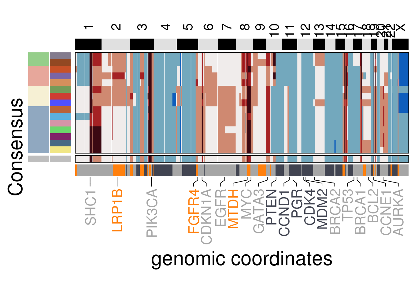

3.3 TN3

# ~~~~~~~~~~~~~~~~~~~~~~~~~~~~~~~~~~~ Tue Nov 24 17:13:42 2020
# Tumors Heatmaps/Consensus/Trees
# ~~~~~~~~~~~~~~~~~~~~~~~~~~~~~~~~~~~ Tue Nov 24 17:13:47 2020

TN3_ploidy <- 3.44

TN3_popseg <- readRDS(here("extdata/popseg/TN3_popseg.rds"))

TN3_popseg_long_ml <- readRDS(here("extdata/merge_levels/TN3_popseg_long_ml.rds"))

TN3_umap <- run_umap(TN3_popseg_long_ml)

## Constructing UMAP embedding.

TN3_clustering <- run_clustering(TN3_umap,
                                 k_snn_major = 65,
                                 k_snn_minor = 17)

## Building SNN graph.

## Running hdbscan.

##  cluster   n    percent
##       c1  67 0.06085377
##       c2  71 0.06448683
##       c3  63 0.05722071
##       c4 450 0.40871935
##       c5  33 0.02997275
##       c6  32 0.02906449
##       c7  77 0.06993642
##       c8 106 0.09627611
##       c9 202 0.18346957

## Done.

TN3_ordered <- order_dataset(popseg_long = TN3_popseg_long_ml,
                             clustering = TN3_clustering)

plot_umap(umap_df = TN3_umap,
          clustering = TN3_clustering)

## Joining, by = "cells"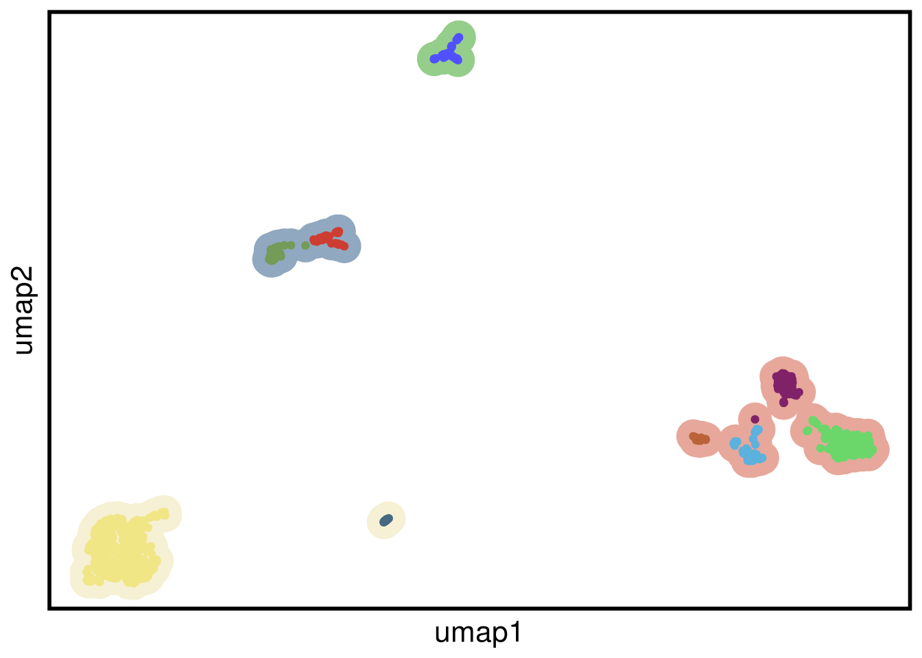

TN3_consensus <- calculate_consensus(df = TN3_ordered$dataset_ordered,
                                     clusters = TN3_ordered$clustering_ordered$subclones)

TN3_gen_classes <- consensus_genomic_classes(TN3_consensus,
                                             ploidy_VAL = TN3_ploidy)

TN3_me_consensus_tree <- run_me_tree(consensus_df = TN3_consensus,
                                     clusters = TN3_clustering,
                                     ploidy_VAL = TN3_ploidy)

TN3_annotation_genes <-
  c(
    "CDKN2C",
    "SHC1",
    "PIK3CA",
    "FGFR4",
    "EGFR",
    "FGFR1",
    "MYC",
    "CDKN2A",
    "GATA3",
    "PTEN",
    "CCND1",
    "CDK4",
    "MDM2",
    "RB1",
    "TP53",
    "BRCA1",
    "BCL2",
    "CCNE1",
    "AURKA",
    "LRP1B"
  )

plot_heatmap(df = TN3_ordered$dataset_ordered,
             ploidy_VAL = TN3_ploidy,
             ploidy_trunc = 2*(round(TN3_ploidy)),
             clusters = TN3_ordered$clustering_ordered,
             genomic_classes = TN3_gen_classes,
             keep_gene = TN3_annotation_genes,
             tree_order = TN3_me_consensus_tree$cs_tree_order,
             show_legend = TRUE)

## 'select()' returned 1:1 mapping between keys and columns

## Warning: The input is a data frame, convert it to the matrix.

plot_consensus_heatmap(df = TN3_consensus,
                       clusters = TN3_ordered$clustering_ordered,
                       ploidy_VAL = TN3_ploidy,
                       ploidy_trunc = 2*(round(TN3_ploidy)),
                       keep_gene = TN3_annotation_genes,
                       tree_order = TN3_me_consensus_tree$cs_tree_order,
                       plot_title = NULL,
                       genomic_classes = TN3_gen_classes)

## Warning: Setting row names on a tibble is deprecated.

## 'select()' returned 1:1 mapping between keys and columns

## Warning: The input is a data frame, convert it to the matrix.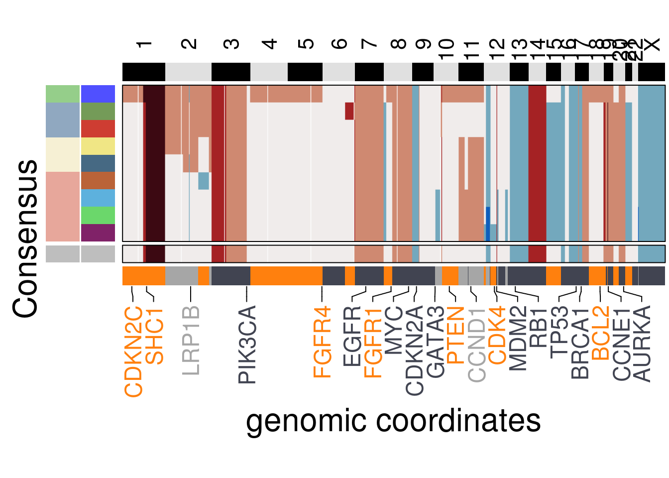

3.4 TN4

# ~~~~~~~~~~~~~~~~~~~~~~~~~~~~~~~~~~~ Tue Nov 24 17:13:42 2020
# Tumors Heatmaps/Consensus/Trees
# ~~~~~~~~~~~~~~~~~~~~~~~~~~~~~~~~~~~ Tue Nov 24 17:13:47 2020

TN4_ploidy <- 3.81

TN4_popseg <- readRDS(here("extdata/popseg/TN4_popseg.rds"))

TN4_popseg_long_ml <- readRDS(here("extdata/merge_levels/TN4_popseg_long_ml.rds"))

TN4_umap <- run_umap(TN4_popseg_long_ml)

## Constructing UMAP embedding.

TN4_clustering <- run_clustering(TN4_umap,
                                 k_snn_major = 75,
                                 k_snn_minor = 17)

## Building SNN graph.

## Running hdbscan.

##  cluster   n    percent
##       c1 255 0.19510329
##      c10  29 0.02218822
##      c11  42 0.03213466
##      c12  46 0.03519510
##      c13  32 0.02448355
##      c14  45 0.03442999
##      c15 220 0.16832441
##      c16  29 0.02218822
##      c17  70 0.05355777
##      c18  37 0.02830910
##      c19  27 0.02065800
##       c2  31 0.02371844
##      c20  36 0.02754399
##      c21  66 0.05049732
##      c22  26 0.01989288
##       c3  31 0.02371844
##       c4  56 0.04284621
##       c5  29 0.02218822
##       c6  66 0.05049732
##       c7  54 0.04131599
##       c8  48 0.03672533
##       c9  32 0.02448355

## Done.

TN4_ordered <- order_dataset(popseg_long = TN4_popseg_long_ml,
                             clustering = TN4_clustering)

plot_umap(umap_df = TN4_umap,
          clustering = TN4_clustering)

## Joining, by = "cells"

TN4_consensus <- calculate_consensus(df = TN4_ordered$dataset_ordered,
                                     clusters = TN4_ordered$clustering_ordered$subclones)

TN4_gen_classes <- consensus_genomic_classes(TN4_consensus,
                                             ploidy_VAL = TN4_ploidy)

TN4_me_consensus_tree <- run_me_tree(consensus_df = TN4_consensus,
                                     clusters = TN4_clustering,
                                     ploidy_VAL = TN4_ploidy)

TN4_annotation_genes <-
  c(
    "CDKN2C",
    "SHC1",
    "PIK3CA",
    "CDKN1A",
    "ESR1",
    "EGFR",
    "MYC",
    "CDKN2A",
    "GATA3",
    "PTEN",
    "MDM2",
    "BRCA2",
    "RB1",
    "TP53",
    "BRCA1",
    "BCL2",
    "CCNE1",
    "NCOA3",
    "AURKA",
    "IGF1R",
    "NCOA1"
  )

plot_heatmap(df = TN4_ordered$dataset_ordered,
             ploidy_VAL = TN4_ploidy,
             ploidy_trunc = 2*(round(TN4_ploidy)),
             clusters = TN4_ordered$clustering_ordered,
             genomic_classes = TN4_gen_classes,
             keep_gene = TN4_annotation_genes,
             tree_order = TN4_me_consensus_tree$cs_tree_order,
             show_legend = TRUE)

## 'select()' returned 1:1 mapping between keys and columns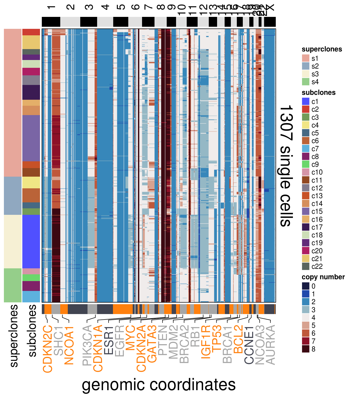

plot_consensus_heatmap(df = TN4_consensus,
                       clusters = TN4_ordered$clustering_ordered,
                       ploidy_VAL = TN4_ploidy,
                       ploidy_trunc = 2*(round(TN4_ploidy)),
                       keep_gene = TN4_annotation_genes,
                       tree_order = TN4_me_consensus_tree$cs_tree_order,
                       plot_title = NULL,
                       genomic_classes = TN4_gen_classes)

## 'select()' returned 1:1 mapping between keys and columns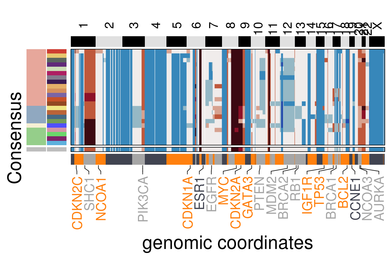

3.5 TN5

# ~~~~~~~~~~~~~~~~~~~~~~~~~~~~~~~~~~~ Tue Nov 24 17:13:42 2020
# Tumors Heatmaps/Consensus/Trees
# ~~~~~~~~~~~~~~~~~~~~~~~~~~~~~~~~~~~ Tue Nov 24 17:13:47 2020

TN5_ploidy <- 2.65

TN5_popseg <- readRDS(here("extdata/popseg/TN5_popseg.rds"))

TN5_popseg_long_ml <- readRDS(here("extdata/merge_levels/TN5_popseg_long_ml.rds"))

TN5_umap <- run_umap(TN5_popseg_long_ml)

## Constructing UMAP embedding.

TN5_clustering <- run_clustering(TN5_umap,
                                 k_snn_major = 41,
                                 k_snn_minor = 17)

## Building SNN graph.

## Running hdbscan.

##  cluster   n    percent
##       c1  52 0.04200323
##       c2  53 0.04281099
##       c3 573 0.46284330
##       c4  27 0.02180937
##       c5 389 0.31421648
##       c6  26 0.02100162
##       c7 118 0.09531502

## Done.

TN5_ordered <- order_dataset(popseg_long = TN5_popseg_long_ml,
                             clustering = TN5_clustering)

plot_umap(umap_df = TN5_umap,
          clustering = TN5_clustering)

## Joining, by = "cells"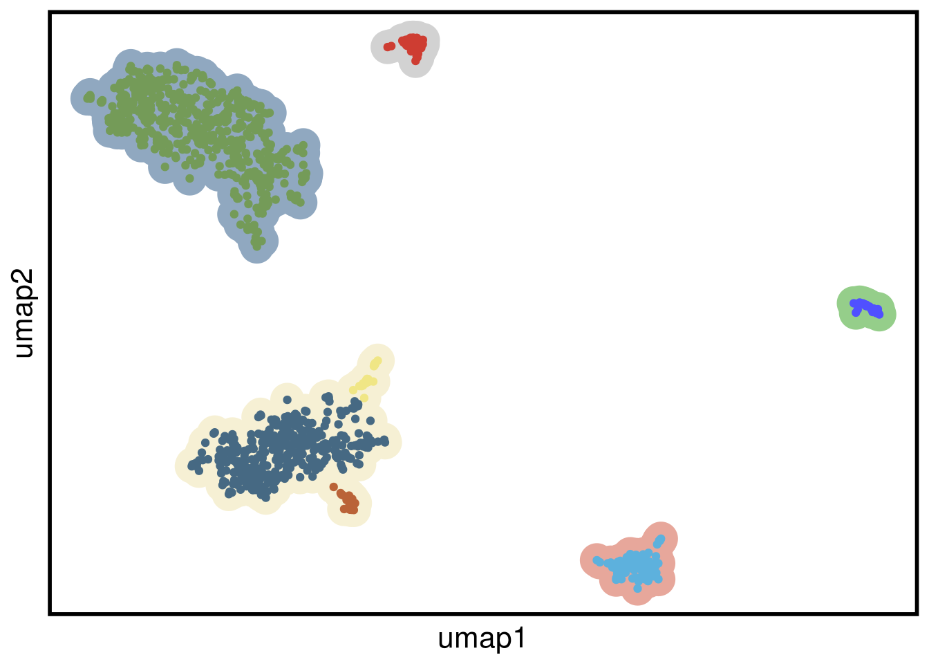

TN5_consensus <- calculate_consensus(df = TN5_ordered$dataset_ordered,
                                     clusters = TN5_ordered$clustering_ordered$subclones)

TN5_gen_classes <- consensus_genomic_classes(TN5_consensus,
                                             ploidy_VAL = TN5_ploidy)

TN5_me_consensus_tree <- run_me_tree(consensus_df = TN5_consensus,
                                     clusters = TN5_clustering,
                                     ploidy_VAL = TN5_ploidy,
                                     rotate_nodes = c(8,10,11))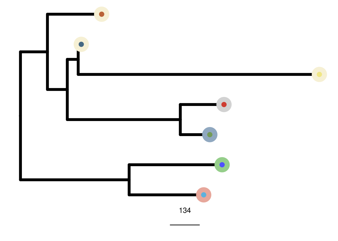

TN5_annotation_genes <-
  c(
    "CDKN2C",
    "GADD45A",
    "SHC1",
    "PIK3CA",
    "FGFR4",
    "EGFR",
    "FGFR1",
    "MYC",
    "CDKN2A",
    "GATA3",
    "PTEN",
    "CCND1",
    "MDM2",
    "BRCA2",
    "RB1",
    "TP53",
    "BRCA1",
    "PPM1D",
    "CCNE1",
    "ERBB2",
    "ESR1"
  )

plot_heatmap(df = TN5_ordered$dataset_ordered,
             ploidy_VAL = TN5_ploidy,
             ploidy_trunc = 2*(round(TN5_ploidy)),
             clusters = TN5_ordered$clustering_ordered,
             genomic_classes = TN5_gen_classes,
             keep_gene = TN5_annotation_genes,
             tree_order = TN5_me_consensus_tree$cs_tree_order,
             show_legend = TRUE)

## 'select()' returned 1:1 mapping between keys and columns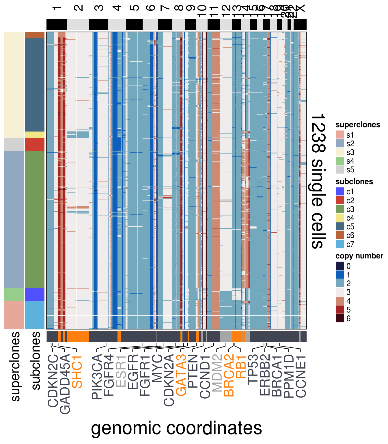

plot_consensus_heatmap(df = TN5_consensus,
                       clusters = TN5_ordered$clustering_ordered,
                       ploidy_VAL = TN5_ploidy,
                       ploidy_trunc = 2*(round(TN5_ploidy)),
                       keep_gene = TN5_annotation_genes,
                       tree_order = TN5_me_consensus_tree$cs_tree_order,
                       plot_title = NULL,
                       genomic_classes = TN5_gen_classes)

## 'select()' returned 1:1 mapping between keys and columns

3.6 TN6

# ~~~~~~~~~~~~~~~~~~~~~~~~~~~~~~~~~~~ Tue Nov 24 17:13:42 2020
# Tumors Heatmaps/Consensus/Trees
# ~~~~~~~~~~~~~~~~~~~~~~~~~~~~~~~~~~~ Tue Nov 24 17:13:47 2020

TN6_ploidy <- 3.17

TN6_popseg <- readRDS(here("extdata/popseg/TN6_popseg.rds"))

TN6_popseg_long_ml <- readRDS(here("extdata/merge_levels/TN6_popseg_long_ml.rds"))

TN6_umap <- run_umap(TN6_popseg_long_ml)

## Constructing UMAP embedding.

TN6_clustering <- run_clustering(TN6_umap,
                                 k_snn_major = 51,
                                 k_snn_minor = 17)

## Building SNN graph.

## Running hdbscan.

##  cluster   n    percent
##       c1  31 0.02249637
##      c10 211 0.15312046
##      c11  31 0.02249637
##      c12  82 0.05950653
##      c13 111 0.08055152
##      c14  37 0.02685051
##      c15  37 0.02685051
##      c16 197 0.14296081
##       c2  25 0.01814224
##       c3  37 0.02685051
##       c4  33 0.02394775
##       c5  42 0.03047896
##       c6  51 0.03701016
##       c7 393 0.28519594
##       c8  18 0.01306241
##       c9  42 0.03047896

## Done.

TN6_ordered <- order_dataset(popseg_long = TN6_popseg_long_ml,
                             clustering = TN6_clustering)

plot_umap(umap_df = TN6_umap,
          clustering = TN6_clustering)

## Joining, by = "cells"

TN6_consensus <- calculate_consensus(df = TN6_ordered$dataset_ordered,
                                     clusters = TN6_ordered$clustering_ordered$subclones)

TN6_gen_classes <- consensus_genomic_classes(TN6_consensus,
                                             ploidy_VAL = TN6_ploidy)

TN6_me_consensus_tree <- run_me_tree(consensus_df = TN6_consensus,
                                     clusters = TN6_clustering,
                                     ploidy_VAL = TN6_ploidy,
                                     rotate_nodes = c(17:20, 22, 29))

TN6_annotation_genes <-
  c(
    "CDKN2C",
    "SHC1",
    "RUVBL1",
    "PIK3CA",
    "CDKN1A",
    "EGFR",
    "FGFR1",
    "CDKN2A",
    "GATA3",
    "PTEN",
    "CDK4",
    "MDM2",
    "BRCA2",
    "RB1",
    "TP53",
    "BRCA1",
    "BCL2",
    "NCOA3",
    "AURKA",
    "GATA3",
    "PGR"
  )

plot_heatmap(df = TN6_ordered$dataset_ordered,
             ploidy_VAL = TN6_ploidy,
             ploidy_trunc = 2*(round(TN6_ploidy)),
             clusters = TN6_ordered$clustering_ordered,
             genomic_classes = TN6_gen_classes,
             keep_gene = TN6_annotation_genes,
             tree_order = TN6_me_consensus_tree$cs_tree_order,
             show_legend = TRUE)

## 'select()' returned 1:1 mapping between keys and columns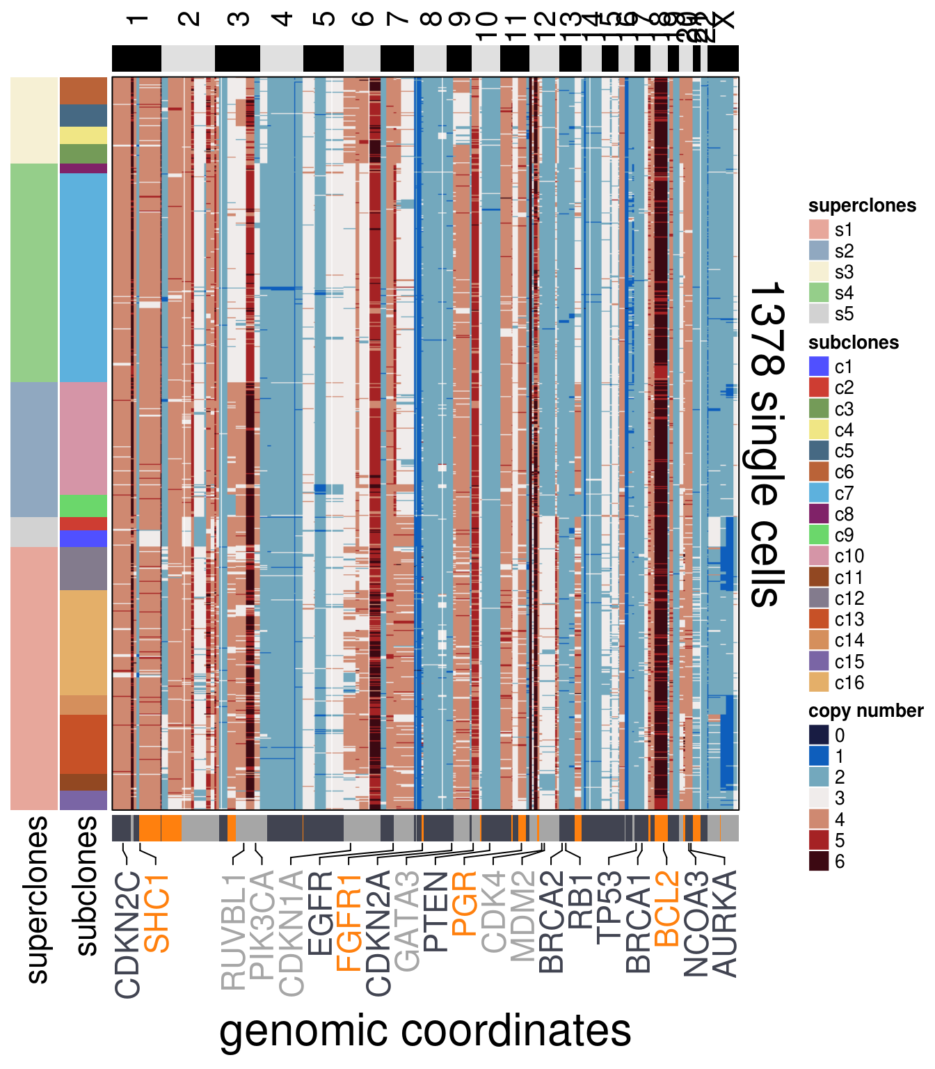

plot_consensus_heatmap(df = TN6_consensus,
                       clusters = TN6_ordered$clustering_ordered,
                       ploidy_VAL = TN6_ploidy,
                       ploidy_trunc = 2*(round(TN6_ploidy)),
                       keep_gene = TN6_annotation_genes,
                       tree_order = TN6_me_consensus_tree$cs_tree_order,
                       plot_title = NULL,
                       genomic_classes = TN6_gen_classes)

## 'select()' returned 1:1 mapping between keys and columns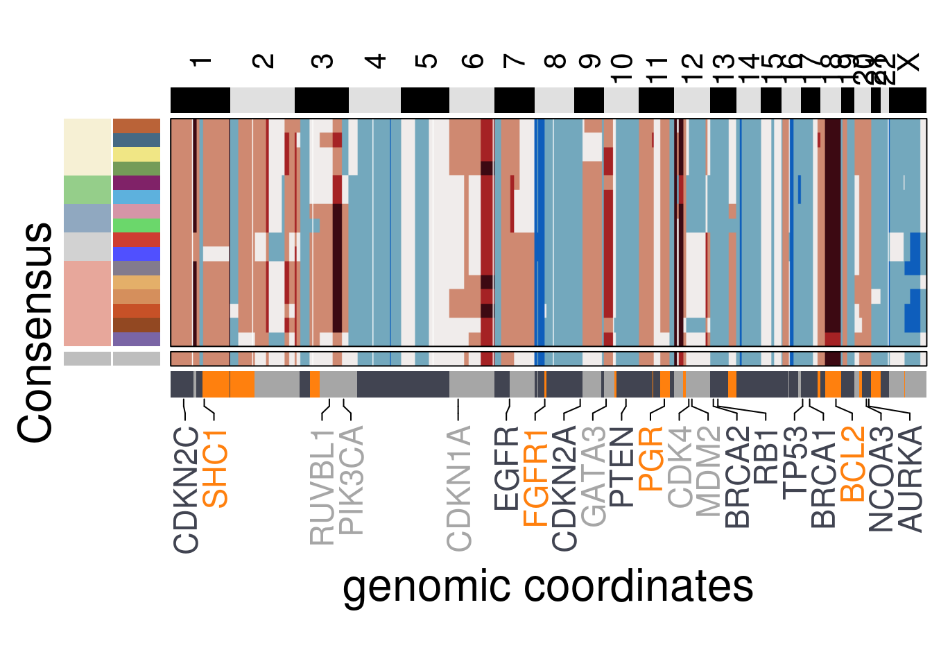

3.7 TN7

# ~~~~~~~~~~~~~~~~~~~~~~~~~~~~~~~~~~~ Tue Nov 24 17:13:42 2020
# Tumors Heatmaps/Consensus/Trees
# ~~~~~~~~~~~~~~~~~~~~~~~~~~~~~~~~~~~ Tue Nov 24 17:13:47 2020

TN7_ploidy <- 3.15

TN7_popseg <- readRDS(here("extdata/popseg/TN7_popseg.rds"))

TN7_popseg_long_ml <- readRDS(here("extdata/merge_levels/TN7_popseg_long_ml.rds"))

TN7_umap <- run_umap(TN7_popseg_long_ml)

## Constructing UMAP embedding.

TN7_clustering <- run_clustering(TN7_umap,
                                 k_snn_major = 35,
                                 k_snn_minor = 17)

## Building SNN graph.

## Running hdbscan.

##  cluster   n    percent
##       c1  17 0.01220388
##      c10  59 0.04235463
##      c11 110 0.07896626
##      c12  63 0.04522613
##      c13 152 0.10911701
##      c14 365 0.26202441
##      c15  30 0.02153625
##      c16  37 0.02656138
##      c17  40 0.02871500
##      c18  53 0.03804738
##       c2 114 0.08183776
##       c3  51 0.03661163
##       c4  45 0.03230438
##       c5  40 0.02871500
##       c6  55 0.03948313
##       c7  56 0.04020101
##       c8  80 0.05743001
##       c9  26 0.01866475

## Done.

TN7_ordered <- order_dataset(popseg_long = TN7_popseg_long_ml,
                             clustering = TN7_clustering)

plot_umap(umap_df = TN7_umap,
          clustering = TN7_clustering)

## Joining, by = "cells"

TN7_consensus <- calculate_consensus(df = TN7_ordered$dataset_ordered,
                                     clusters = TN7_ordered$clustering_ordered$subclones)

TN7_gen_classes <- consensus_genomic_classes(TN7_consensus,
                                             ploidy_VAL = TN7_ploidy)

TN7_me_consensus_tree <- run_me_tree(consensus_df = TN7_consensus,
                                     clusters = TN7_clustering,
                                     ploidy_VAL = TN7_ploidy,
                                     rotate_nodes = c(26, 27))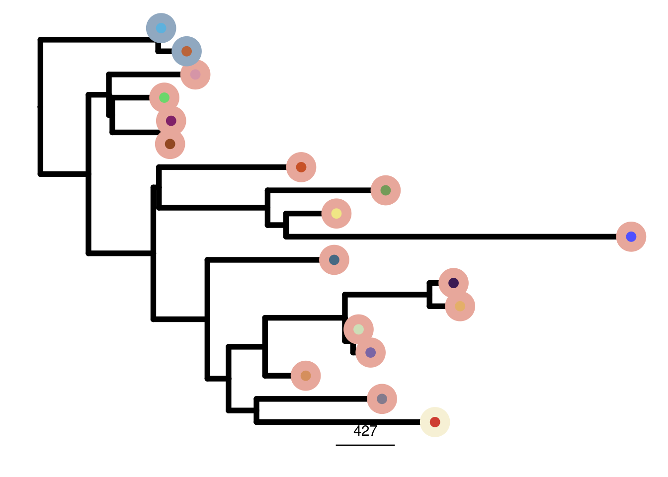

TN7_annotation_genes <-
  c(
    "CDKN2C",
    "SHC1",
    "RUVBL1",
    "PIK3CA",
    "CDKN1A",
    "EGFR",
    "FGFR1",
    "CDKN2A",
    "GATA3",
    "PTEN",
    "CDK4",
    "MDM2",
    "BRCA2",
    "RB1",
    "TP53",
    "BRCA1",
    "BCL2",
    "NCOA3",
    "AURKA",
    "GATA3",
    "PGR"
  )

plot_heatmap(df = TN7_ordered$dataset_ordered,
             ploidy_VAL = TN7_ploidy,
             ploidy_trunc = 2*(round(TN7_ploidy)),
             clusters = TN7_ordered$clustering_ordered,
             genomic_classes = TN7_gen_classes,
             keep_gene = TN7_annotation_genes,
             tree_order = TN7_me_consensus_tree$cs_tree_order,
             show_legend = TRUE)

## 'select()' returned 1:1 mapping between keys and columns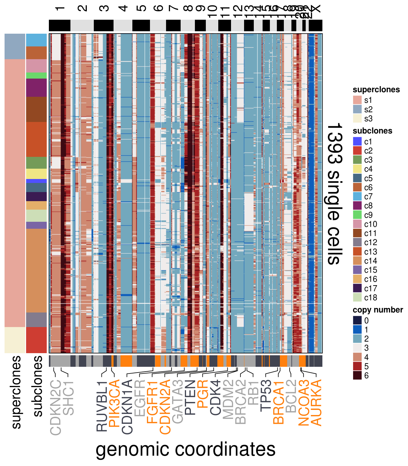

plot_consensus_heatmap(df = TN7_consensus,
                       clusters = TN7_ordered$clustering_ordered,
                       ploidy_VAL = TN7_ploidy,
                       ploidy_trunc = 2*(round(TN7_ploidy)),
                       keep_gene = TN7_annotation_genes,
                       tree_order = TN7_me_consensus_tree$cs_tree_order,
                       plot_title = NULL,
                       genomic_classes = TN7_gen_classes)

## 'select()' returned 1:1 mapping between keys and columns

3.8 TN8

# ~~~~~~~~~~~~~~~~~~~~~~~~~~~~~~~~~~~ Tue Nov 24 17:13:42 2020
# Tumors Heatmaps/Consensus/Trees
# ~~~~~~~~~~~~~~~~~~~~~~~~~~~~~~~~~~~ Tue Nov 24 17:13:47 2020

TN8_ploidy <- 3.95

TN8_popseg <- readRDS(here("extdata/popseg/TN8_popseg.rds"))

TN8_popseg_long_ml <- readRDS(here("extdata/merge_levels/TN8_popseg_long_ml.rds"))

TN8_umap <- run_umap(TN8_popseg_long_ml)

## Constructing UMAP embedding.

TN8_clustering <- run_clustering(TN8_umap,
                                 k_snn_major = 43,
                                 k_snn_minor = 17)

## Building SNN graph.

## Running hdbscan.

##  cluster   n    percent
##       c1  38 0.03104575
##      c10  29 0.02369281
##      c11  52 0.04248366
##      c12  45 0.03676471
##      c13  43 0.03513072
##      c14  44 0.03594771
##      c15 263 0.21486928
##       c2  54 0.04411765
##       c3  96 0.07843137
##       c4  55 0.04493464
##       c5  88 0.07189542
##       c6  22 0.01797386
##       c7  35 0.02859477
##       c8 325 0.26552288
##       c9  35 0.02859477

## Done.

TN8_ordered <- order_dataset(popseg_long = TN8_popseg_long_ml,
                             clustering = TN8_clustering)

plot_umap(umap_df = TN8_umap,
          clustering = TN8_clustering)

## Joining, by = "cells"

TN8_consensus <- calculate_consensus(df = TN8_ordered$dataset_ordered,
                                     clusters = TN8_ordered$clustering_ordered$subclones)

TN8_gen_classes <- consensus_genomic_classes(TN8_consensus,
                                             ploidy_VAL = TN8_ploidy)

TN8_me_consensus_tree <- run_me_tree(consensus_df = TN8_consensus,
                                     clusters = TN8_clustering,
                                     ploidy_VAL = TN8_ploidy,
                                     rotate_nodes = c(17,18, 25, 29))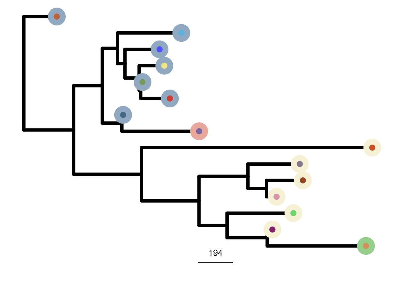

TN8_annotation_genes <-
  c(
    "CDKN2C",
    "SHC1",
    "ESR1",
    "MTDH",
    "MYC",
    "GATA3",
    "PTEN",
    "PGR",
    "MDM2",
    "BRCA2",
    "RB1",
    "BCL2",
    "NCOA3",
    "AURKA",
    "CHEK2"
  )

plot_heatmap(df = TN8_ordered$dataset_ordered,
             ploidy_VAL = TN8_ploidy,
             ploidy_trunc = 2*(round(TN8_ploidy)),
             clusters = TN8_ordered$clustering_ordered,
             genomic_classes = TN8_gen_classes,
             keep_gene = TN8_annotation_genes,
             tree_order = TN8_me_consensus_tree$cs_tree_order,
             show_legend = TRUE)

## 'select()' returned 1:1 mapping between keys and columns

plot_consensus_heatmap(df = TN8_consensus,
                       clusters = TN8_ordered$clustering_ordered,
                       ploidy_VAL = TN8_ploidy,
                       ploidy_trunc = 2*(round(TN8_ploidy)),
                       keep_gene = TN8_annotation_genes,
                       tree_order = TN8_me_consensus_tree$cs_tree_order,
                       plot_title = NULL,
                       genomic_classes = TN8_gen_classes)

## 'select()' returned 1:1 mapping between keys and columns

3.9 Clones barplot

n_clones_tumors <- tibble(
  sample = rep(c(
    "TN1",
    "TN2",
    "TN3",
    "TN4",
    "TN5",
    "TN6",
    "TN7",
    "TN8"
  ),2),
  n_clones = c(
    length(unique(TN1_clustering$superclones)),
    length(unique(TN2_clustering$superclones)),
    length(unique(TN3_clustering$superclones)),
    length(unique(TN4_clustering$superclones)),
    length(unique(TN5_clustering$superclones)),
    length(unique(TN6_clustering$superclones)),
    length(unique(TN7_clustering$superclones)),
    length(unique(TN8_clustering$superclones)),
    length(unique(TN1_clustering$subclones)),
    length(unique(TN2_clustering$subclones)),
    length(unique(TN3_clustering$subclones)),
    length(unique(TN4_clustering$subclones)),
    length(unique(TN5_clustering$subclones)),
    length(unique(TN6_clustering$subclones)),
    length(unique(TN7_clustering$subclones)),
    length(unique(TN8_clustering$subclones))
  ),
  group = c(
    rep("superclones",8),
    rep("subclones", 8)
  )
) 

p_clones_tumors <- n_clones_tumors %>%
  ggplot() +
  geom_col(
    aes(
      x = sample,
      y = n_clones,
      fill = fct_relevel(group, c("superclones",
                                  "subclones"))
    ),
    position = "dodge"
  ) +
  theme_classic() +
  my_theme +
  theme(axis.text.x = element_text(angle = 90, vjust = .5)) +
  scale_y_continuous(
    breaks = scales::pretty_breaks(n = 10),
    limits = c(0, 22),
    expand = c(0, 0)
  ) +
  paletteer::scale_fill_paletteer_d("yarrr::info") +
  xlab("") +
  ylab("number of clones")

p_clones_tumors

3.10 Shannon diversity

shan <- function(data, indices) {
  data_ind <- data[indices]
  prop <- janitor::tabyl(data_ind) %>% pull(percent) 
  div <- -sum(prop*log(prop))
  return(div)
}

TN1_proportions <- janitor::tabyl(TN1_clustering$subclones) %>% pull(percent)
TN2_proportions <- janitor::tabyl(TN2_clustering$subclones) %>% pull(percent)
TN3_proportions <- janitor::tabyl(TN3_clustering$subclones) %>% pull(percent)
TN4_proportions <- janitor::tabyl(TN4_clustering$subclones) %>% pull(percent)
TN5_proportions <- janitor::tabyl(TN5_clustering$subclones) %>% pull(percent)
TN6_proportions <- janitor::tabyl(TN6_clustering$subclones) %>% pull(percent)
TN7_proportions <- janitor::tabyl(TN7_clustering$subclones) %>% pull(percent)
TN8_proportions <- janitor::tabyl(TN8_clustering$subclones) %>% pull(percent)

TN1_diver <- -sum(TN1_proportions*log(TN1_proportions))
TN2_diver <- -sum(TN2_proportions*log(TN2_proportions))
TN3_diver <- -sum(TN3_proportions*log(TN3_proportions))
TN4_diver <- -sum(TN4_proportions*log(TN4_proportions))
TN5_diver <- -sum(TN5_proportions*log(TN5_proportions))
TN6_diver <- -sum(TN6_proportions*log(TN6_proportions))
TN7_diver <- -sum(TN7_proportions*log(TN7_proportions))
TN8_diver <- -sum(TN8_proportions*log(TN8_proportions))

boot_TN1 <- boot::boot(TN1_clustering$subclones, statistic = shan,  R = 3000)
boot_TN1_ci <- boot::boot.ci(boot_TN1)

boot_TN2 <- boot::boot(TN2_clustering$subclones, statistic = shan,  R = 3000)
boot_TN2_ci <- boot::boot.ci(boot_TN2)

boot_TN3 <- boot::boot(TN3_clustering$subclones, statistic = shan,  R = 3000)
boot_TN3_ci <- boot::boot.ci(boot_TN3)

boot_TN4 <- boot::boot(TN4_clustering$subclones, statistic = shan,  R = 3000)
boot_TN4_ci <- boot::boot.ci(boot_TN4)

boot_TN5 <- boot::boot(TN5_clustering$subclones, statistic = shan,  R = 3000)
boot_TN5_ci <- boot::boot.ci(boot_TN5)

boot_TN6 <- boot::boot(TN6_clustering$subclones, statistic = shan,  R = 3000)
boot_TN6_ci <- boot::boot.ci(boot_TN6)

boot_TN7 <- boot::boot(TN7_clustering$subclones, statistic = shan,  R = 3000)
boot_TN7_ci <- boot::boot.ci(boot_TN7)

boot_TN8 <- boot::boot(TN8_clustering$subclones, statistic = shan,  R = 3000)
boot_TN8_ci <- boot::boot.ci(boot_TN8)


div_table <- tibble(
  sample = c("TN1",
             "TN2",
             "TN3",
             "TN4",
             "TN5",
             "TN6",
             "TN7",
             "TN8"),
  shannon_index = c(
    TN1_diver,
    TN2_diver,
    TN3_diver,
    TN4_diver,
    TN5_diver,
    TN6_diver,
    TN7_diver,
    TN8_diver
  ),
  lci = c(
    boot_TN1_ci$normal[2],
    boot_TN2_ci$normal[2],
    boot_TN3_ci$normal[2],
    boot_TN4_ci$normal[2],
    boot_TN5_ci$normal[2],
    boot_TN6_ci$normal[2],
    boot_TN7_ci$normal[2],
    boot_TN8_ci$normal[2]
  ),
  uci = c(
    boot_TN1_ci$normal[3],
    boot_TN2_ci$normal[3],
    boot_TN3_ci$normal[3],
    boot_TN4_ci$normal[3],
    boot_TN5_ci$normal[3],
    boot_TN6_ci$normal[3],
    boot_TN7_ci$normal[3],
    boot_TN8_ci$normal[3]
  )
)

# error bar = 95% confidence interval
p_tumors_diver <- div_table %>%
  ggplot() +
  geom_errorbar(aes(
    x = fct_reorder(sample, shannon_index),
    ymin = lci,
    ymax = uci
  ),
  width = .1,
  size = 2) +
  geom_point(aes(
    x = fct_reorder(sample, shannon_index),
    y = shannon_index,
    color = sample
  ), size = 4) +
  theme_classic() +
  my_theme +
  theme(legend.position = "none",
        axis.text.x = element_text(
          angle = 90,
          vjust = 0.5,
          hjust = 1
        )) +
  scale_y_continuous(breaks = scales::pretty_breaks(n = 12)) +
  scale_color_manual(values = c(rcartocolor::carto_pal(8, "Safe"))) +
  ylab("shannon diversity index") +
  xlab("")

p_tumors_diver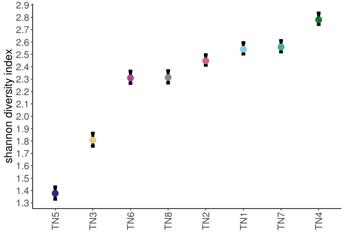

3.11 Gains/Losses plot

TN1_alt_perc <-
  gain_loss_percentage(consensus = TN1_consensus,
                       ploidy_VAL = TN1_ploidy,
                       sample = "TN1")

TN2_alt_perc <-
  gain_loss_percentage(consensus = TN2_consensus,
                       ploidy = TN2_ploidy,
                       sample = "TN2")

TN3_alt_perc <-
  gain_loss_percentage(consensus = TN3_consensus,
                       ploidy = TN3_ploidy,
                       sample = "TN3")

TN4_alt_perc <-
  gain_loss_percentage(consensus = TN4_consensus,
                       ploidy = TN4_ploidy,
                       sample = "TN4")

TN5_alt_perc <-
  gain_loss_percentage(consensus = TN5_consensus,
                       ploidy = TN5_ploidy,
                       sample = "TN5")

TN6_alt_perc <-
  gain_loss_percentage(consensus = TN6_consensus,
                       ploidy = TN6_ploidy,
                       sample = "TN6")

TN7_alt_perc <-
  gain_loss_percentage(consensus = TN7_consensus,
                       ploidy = TN7_ploidy,
                       sample = "TN7")

TN8_alt_perc <-
  gain_loss_percentage(consensus = TN8_consensus,
                       ploidy = TN8_ploidy,
                       sample = "TN8")


all_tumors_gainloss_percentage <- 
  bind_rows(TN2_alt_perc,
            TN3_alt_perc,
            TN4_alt_perc,
            TN1_alt_perc,
            TN5_alt_perc,
            TN6_alt_perc,
            TN7_alt_perc,
            TN8_alt_perc
            ) %>% 
  dplyr::rename(percent = n)

p_gain_loss <- ggplot() +
  geom_col(data = all_tumors_gainloss_percentage, 
           aes(x = fct_relevel(clone, rev(unique(gtools::mixedsort(all_tumors_gainloss_percentage$clone)))),
               y = percent,
               fill = class
           ),
           color = "black") +
  facet_wrap(vars(sample), ncol = 4, scales = "free_y") +
  scale_fill_manual(values = c("ground_state" = "white",
                               "gain" = "firebrick3",
                               "loss" = "steelblue"),
                    label = c("loss",
                              "neutral",
                              "gain"),
                    breaks = c("loss",
                               "ground_state",
                               "gain")) +
  theme_cowplot() +
    theme(strip.background = element_rect(fill = "white"),
        legend.title = element_blank(),
        legend.position = "top",
        axis.text = element_text(size = 10)) +
  coord_flip() +
  xlab("") 
  # ggtitle("Percentage of gain_loss per subclone")

p_gain_loss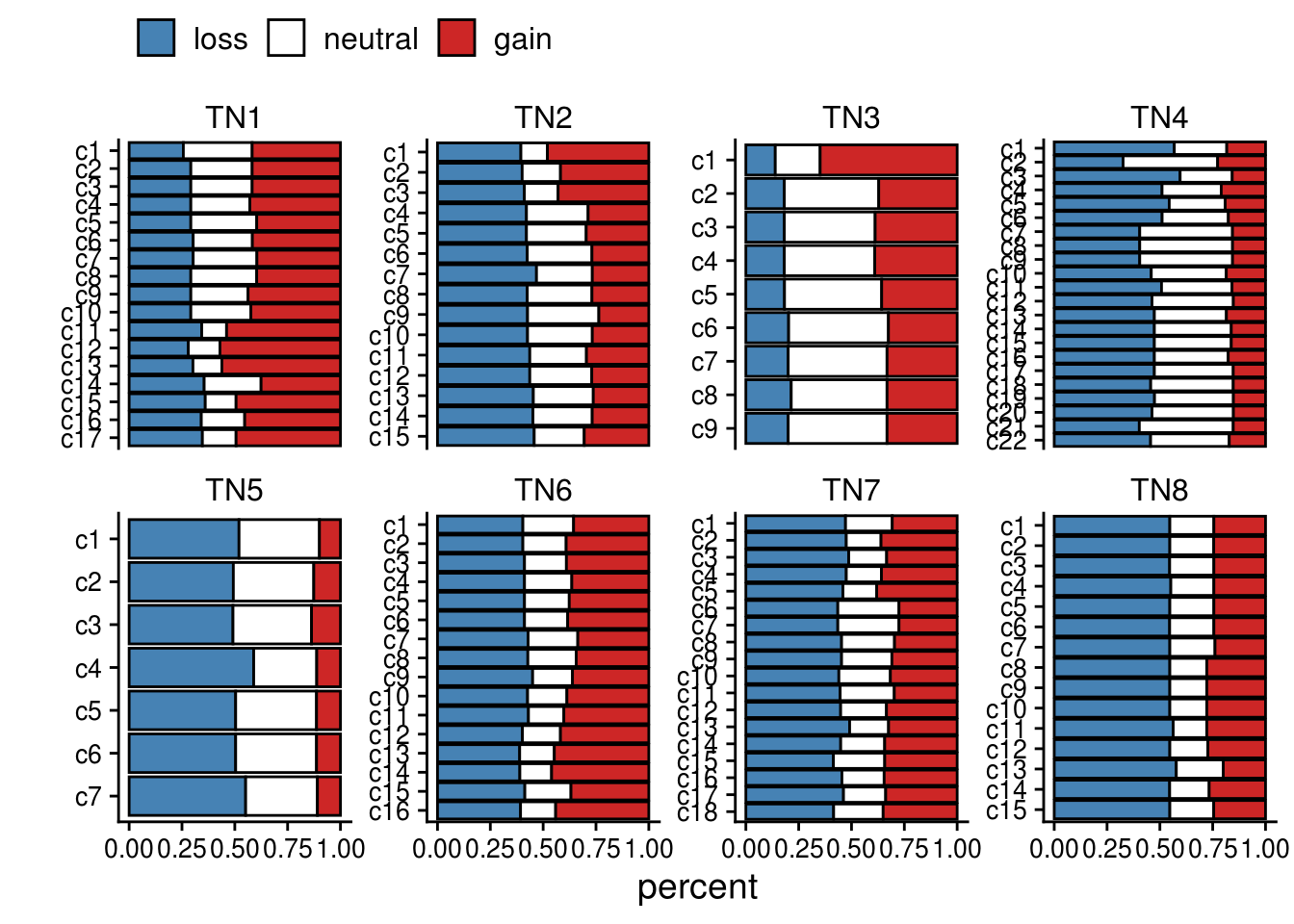

3.12 Genomic classes plots

3.12.1 Counts

TN1_seg_length <- calc_genclass_length(TN1_gen_classes,
                                       popseg = TN1_popseg,
                                       popseg_long = TN1_popseg_long_ml) %>% 
  mutate(sample = "TN1")

TN2_seg_length <- calc_genclass_length(TN2_gen_classes,
                                       popseg = TN2_popseg,
                                       popseg_long = TN2_popseg_long_ml) %>% 
  mutate(sample = "TN2")

TN3_seg_length <- calc_genclass_length(TN3_gen_classes,
                                       popseg = TN3_popseg,
                                       popseg_long = TN3_popseg_long_ml) %>% 
  mutate(sample = "TN3")

TN4_seg_length <- calc_genclass_length(TN4_gen_classes,
                                       popseg = TN4_popseg,
                                       popseg_long = TN4_popseg_long_ml) %>% 
  mutate(sample = "TN4")

TN5_seg_length <- calc_genclass_length(TN5_gen_classes,
                                       popseg = TN5_popseg,
                                       popseg_long = TN5_popseg_long_ml) %>% 
  mutate(sample = "TN5")

TN6_seg_length <- calc_genclass_length(TN6_gen_classes,
                                       popseg = TN6_popseg,
                                       popseg_long = TN6_popseg_long_ml) %>% 
  mutate(sample = "TN6")

TN7_seg_length <- calc_genclass_length(TN7_gen_classes,
                                       popseg = TN7_popseg,
                                       popseg_long = TN7_popseg_long_ml) %>% 
  mutate(sample = "TN7")

TN8_seg_length <- calc_genclass_length(TN8_gen_classes,
                                       popseg = TN8_popseg,
                                       popseg_long = TN8_popseg_long_ml) %>% 
  mutate(sample = "TN8")

df_cna <- bind_rows(TN1_seg_length,
                    TN2_seg_length,
                    TN3_seg_length,
                    TN4_seg_length,
                    TN5_seg_length,
                    TN6_seg_length,
                    TN7_seg_length,
                    TN8_seg_length)

p_count_cna <- df_cna %>%
  dplyr::group_by(sample) %>%
  dplyr::distinct(seg_index, .keep_all = TRUE) %>% 
  dplyr::count(class) %>% 
  dplyr::mutate(class = fct_relevel(class,
                                    c("uCNA",
                                      "sCNA",
                                      "cCNA"))) %>%
  ggplot()  +
  geom_bar(
    aes(x =  sample,
        y = n,
        fill = class),
    position = "stack",
    stat = "identity",
    width = .6
  ) +
  scale_fill_manual(
    values = c(
      "cCNA" = "#414451",
      "sCNA" = "#A5ACAF",
      "uCNA" = "#FF800E"
    ),
    breaks = c("cCNA",
               "sCNA",
               "uCNA"),
    labels = c("cCNA",
               "sCNA",
               "uCNA")
  ) +
  scale_y_continuous(breaks = scales::pretty_breaks(n = 15),
                     expand = c(0, 0)) +
  theme_classic() +
  my_theme +
  theme(legend.position = 'top',
        axis.text.x = element_text(angle = 90,
                                   vjust = .5,
                                   hjust = 1),
        axis.text = element_text(color = 'black')) +
  xlab("") +
  ylab("CNA class count")

p_count_cna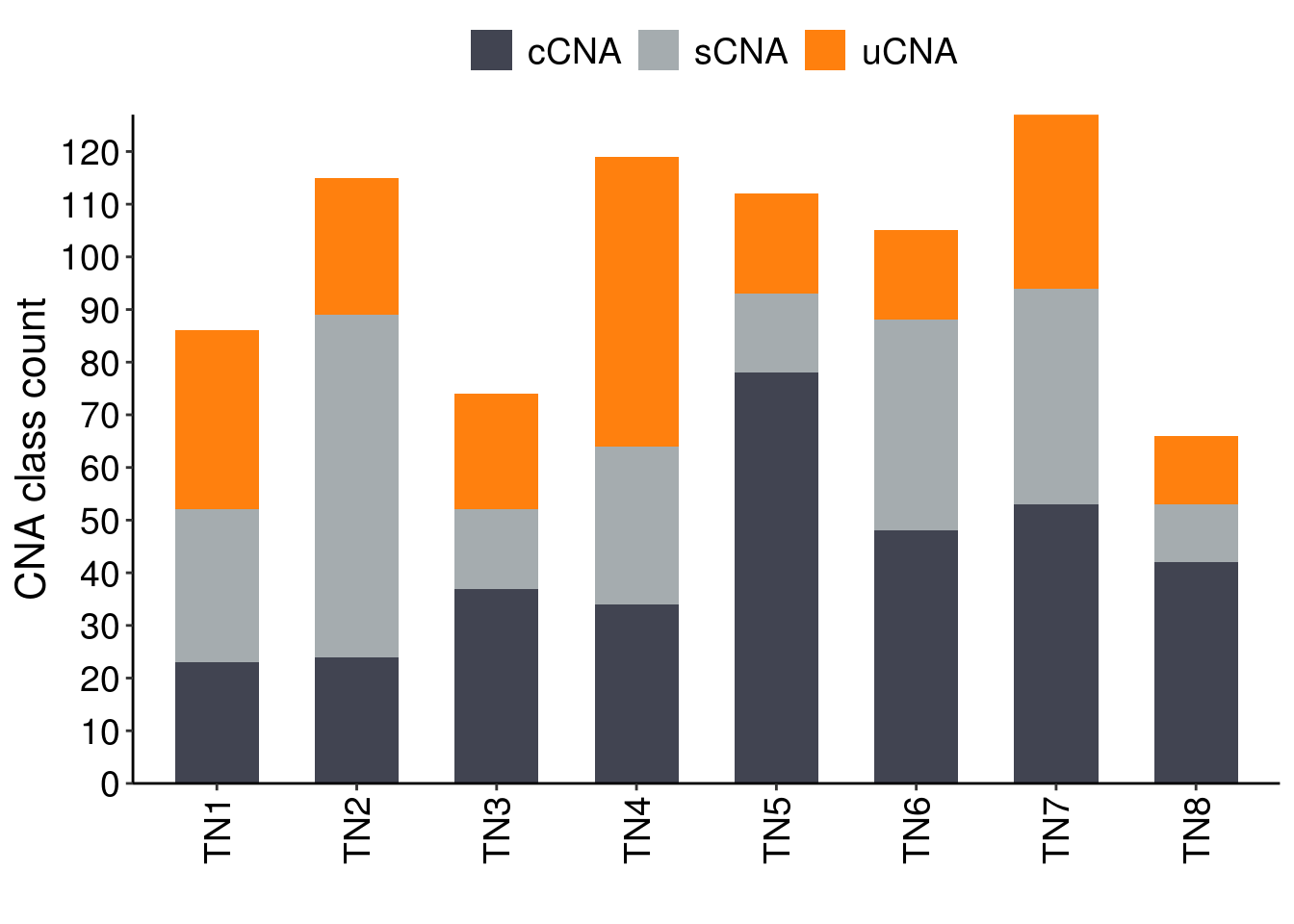

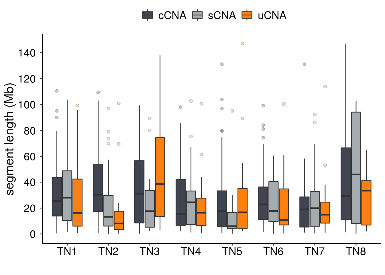
3.12.2 Segment length

p_seg_box <- df_cna %>%
    dplyr::group_by(sample) %>%
  dplyr::distinct(seg_index, .keep_all = TRUE) %>% 
  dplyr::mutate(class = fct_relevel(class,
                                    c("cCNA",
                                      "sCNA",
                                      "uCNA"))) %>%
  ggplot() +
  geom_boxplot(
    aes(x = sample,
        y = seg_length,
        fill = class),
    outlier.shape = 21,
    outlier.alpha = .3
  ) +
  scale_fill_manual(
    values = c(
      "cCNA" = "#414451",
      "sCNA" = "#A5ACAF",
      "uCNA" = "#FF800E"
    ),
    breaks = c("cCNA",
               "sCNA",
               "uCNA"),
    labels = c("cCNA",
               "sCNA",
               "uCNA")
  ) +
  theme_classic() +
  my_theme +
  theme(axis.text = element_text(color = "black")) +
  scale_y_continuous(
    breaks = scales::pretty_breaks(n = 10),
    labels = scales::unit_format(unit = "",
                                 scale = 1e-6)
  ) +
  xlab("") +
  ylab("segment length (Mb)")

p_seg_box

source(here("R/setup.R"))
source(here("R/calc_sctree_dists.R"))
source(here("R/plot_sctree.R"))